A Toy Example with Translational Distance Models
The following tutorial is based on a question originally posed by Heiko Paulheim on the PyKEEN Issue Tracker #97.
Given the following toy example comprising three entities in a triangle, a translational distance model like
pykeen.models.TransE should be able to exactly learn the geometric structure.
Head |
Relation |
Tail |
|---|---|---|
Brussels |
locatedIn |
Belgium |
Belgium |
partOf |
EU |
EU |
hasCapital |
Brussels |
from pykeen.pipeline import pipeline

tf = ...
results = pipeline(
    training=tf,
    testing=...,
    model="TransE",
    model_kwargs=dict(embedding_dim=2),
    random_seed=1,
    device="cpu",
)
results.plot()
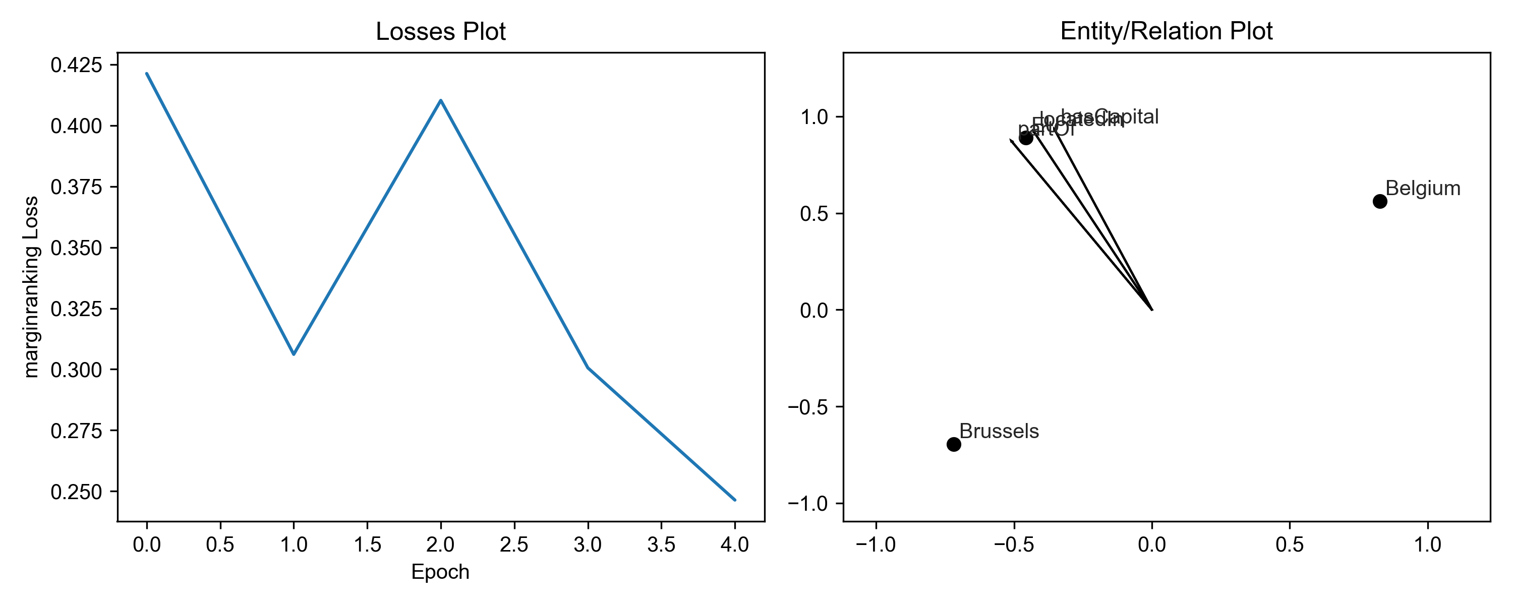
First, check if the model is converging using results.plot_losses. Qualitatively, this means that the loss is
smoothly decreasing and eventually evening out. If the model does not decrease, you might need to tune some parameters
with the optimizer_kwargs and training_kwargs to the pipeline() function.
For example, you can decrease the optimizer’s learning rate to make the loss curve less bumpy. Second, you can increase the number of epochs during training.
results = pipeline(
    training=tf,
    testing=...,
    model="TransE",
    model_kwargs=dict(embedding_dim=2),
    optimizer_kwargs=dict(lr=1.0e-1),
    training_kwargs=dict(num_epochs=128, use_tqdm_batch=False),
    evaluation_kwargs=dict(use_tqdm=False),
    random_seed=1,
    device="cpu",
)
results.plot()
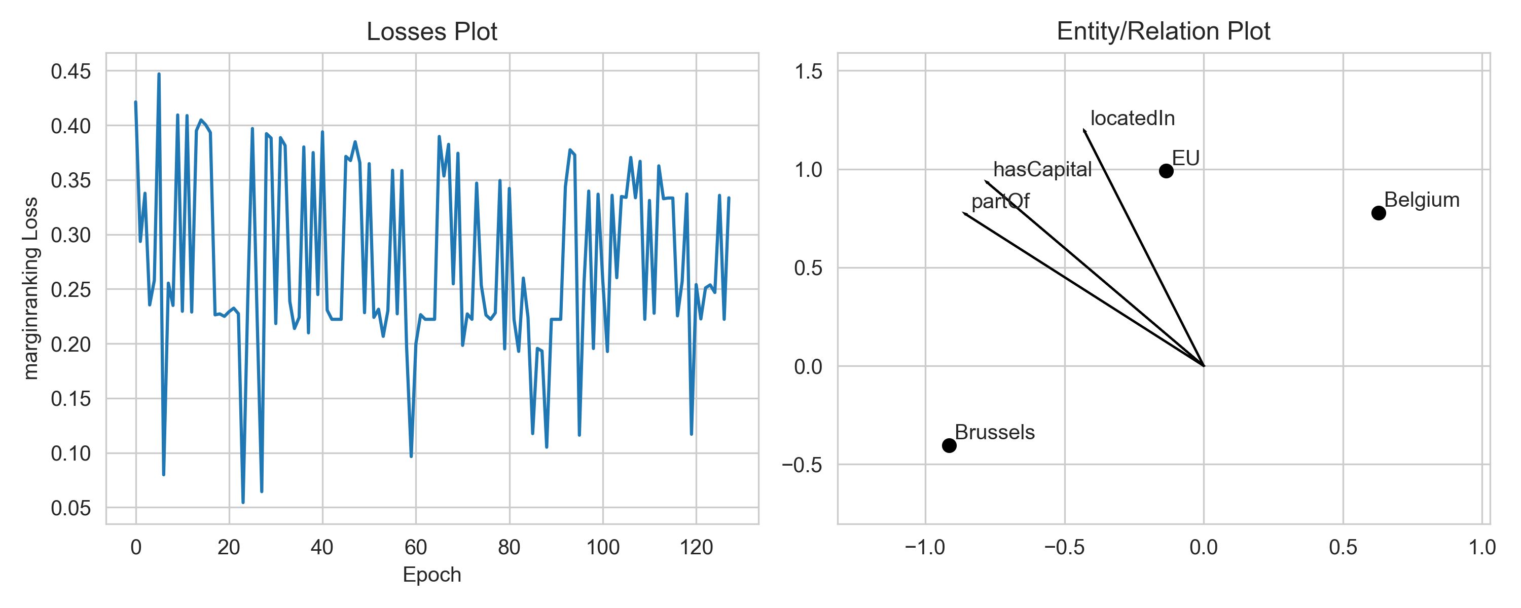
Please notice that there is some stochasticity in the training, since we sample negative examples for positive ones. Thus, the loss may fluctuate naturally. To better see the trend, you can smooth the loss by averaging over a window of epochs.
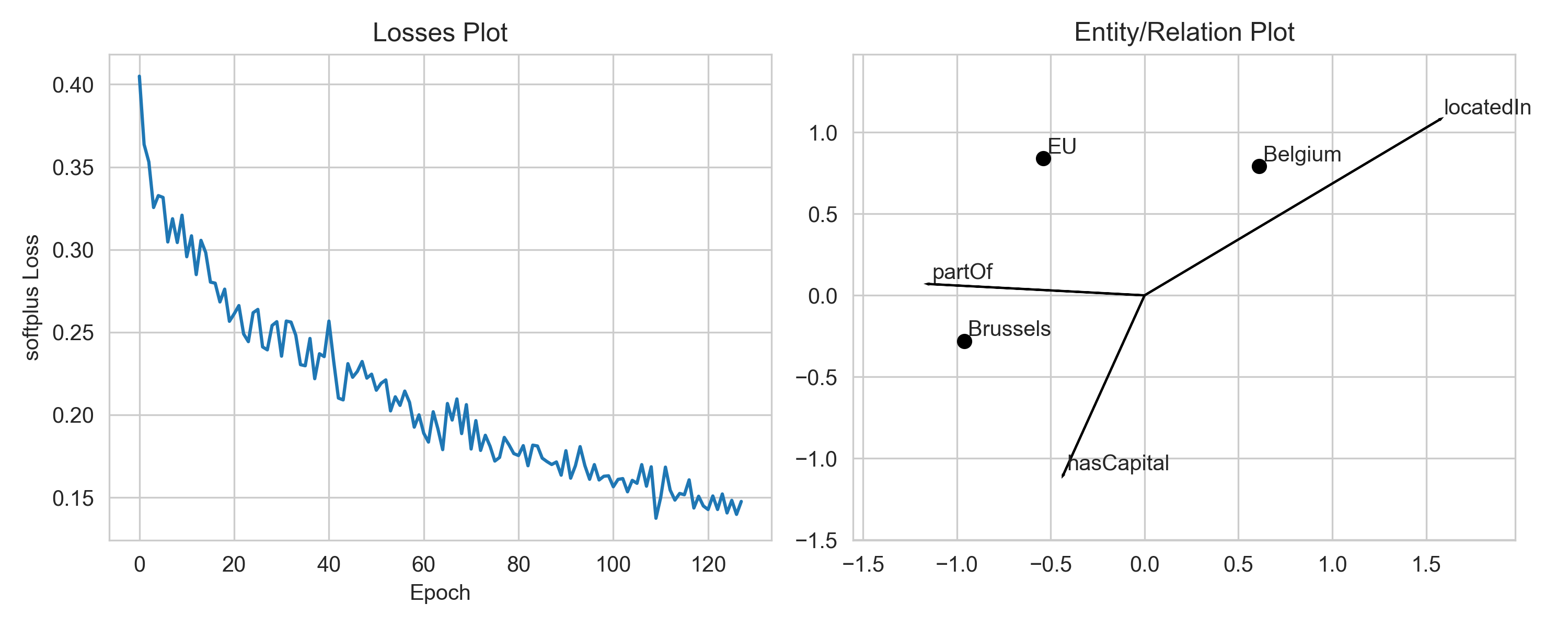
We use a margin-based loss with TransE by default. Thus, it suffices if the model predicts scores such that the scores
of positive triples and negative triples are at least one margin apart. Once the model has reached this state, if will
not improve further upon these examples, as the embeddings are “good enough”. Hence, an optimal solution with
margin-based loss might not look like the exact geometric solution. If you want to change that you can switch to a loss
function which does not use a margin, e.g. the softplus loss. You can do this by passing loss="softplus" to the
pipeline.
toy_results = pipeline(
    training=tf,
    testing=...,
    model="TransE",
    loss="softplus",
    model_kwargs=dict(embedding_dim=2),
    optimizer_kwargs=dict(lr=1.0e-1),
    training_kwargs=dict(num_epochs=128, use_tqdm_batch=False),
    evaluation_kwargs=dict(use_tqdm=False),
    random_seed=1,
    device="cpu",
)
results.plot()
There was a lot of interesting follow-up discussion at !99 during which this code was implemented for re-use. One of the interesting points is that the relation plot is only applicable for translational distance models like TransE. Further, when models whose embeddings are higher than 2, a dimensionality reduction method must be used. For this, one of many of the tools from scikit-learn can be chosen. However, to make sure that the entities and relations are projected on the same axis, the dimensionality reduction model is first trained on the entity embeddings, then applied on both the entity embeddings and relation embeddings. Further, non-linear models like KPCA should not be used when plotting relations, since these _should_ correspond to linear transformations in embedding space.